Vol.32 (Jun) 2022 | Article no.14 2022
Nuclear theory research is undergoing a renaissance owing to the recent advancements in the high-performance computing. As nucleus is a quantum many-body system with complicated interparticle interactions, initial theoretical developments were predominantly based on different phenomenological models derived with the help of numerous simplifying assumptions. Although appropriate nuclear many-body theories were formulated, these were hardly adopted in practical applications because of computational limitations. However, since the last decade, this scenario has changed as a result of rapid improvements in the computational power and the associated numerical techniques. Realistic microscopic theories with superior predictive power are now routinely used even for systems which are far beyond the laboratory reach. This review discusses recent achievements in the microscopic theories of large amplitude nuclear dynamics. Particularly, after a succinct historical introduction, emphasis is given to the discussions on the microscopic modelling of nuclear fission dynamics. Also, related future directions are mentioned in brief.
The atomic nucleus is a quantum many-body system with non-trivial internucleonic interactions, which are still unknown to a large extent. Hence, it is a daunting challenge to model the dynamics of an excited nucleus by employing an exact microscopic theory [1]. Nuclear fission process provides a suitable platform to study large-amplitude collective dynamics in nuclei, and the pertaining theoretical model can reveal the nature of the underlying interactions by correlating them with fission observables. Two primary measurable quantities in fission decay are the fission yields and the decay half-life. Depending on the intrinsic properties of a nucleus, fission may occur without any external perturbation. This is known as spontaneous fission (SF). Theoretical understanding of SF is based on the quantum tunnelling phenomena [2]. On the other hand, fission can be induced by exciting a nucleus through different reaction mechanisms. Such a decay process is usually faster than SF, and it can be visualized as diffusion of nuclear shape, similar to the motion of a Brownian particle in a heat bath [3]. Therefore, a comprehensive theoretical description of nuclear fission encompasses different domains of physics ranging from simple classical mechanics to many-body quantum theory. In the present review, I will focus only on the theoretical aspects that deal with the microscopic modelling of fission dynamics. These are mainly relevant to the two categories of fission decay: SF and low-energy fission induced by thermal neutrons. In short, the second category is known as the thermal fission.
In 1934, Enrico Fermi [4] discovered that certain heavy nuclei can capture neutrons to form new radioactive isotopes of higher masses and charge numbers than hitherto known. Decay of these excited nuclei was investigated experimentally and multiple half-lives were detected indicating the presence of unknown processes other than β-decay. The pursuit of these investigations led Meitner and Frisch [5] to the discovery of fission in 1939. Subsequently, considerable theoretical [6, 7] and experimental [8, 9] advancements took place. Nevertheless, even after eight decades of its discovery, fission continues to be an important field of research because of its extensive applications in basic sciences and nuclear engineering.
According to the present-day understanding, rapid neutron capture process (or r-process) is responsible for producing more than half of all the elements heavier than iron. This process requires very-neutron-rich astrophysical environment, which can be found in the tidal ejecta of neutron stars. In the r-process, fission determines the endpoint where the neutron-rich heavy element bifurcates as the competing β-decay channel is either forbidden or less probable compared to the fission mode [10]. For example, the SF half-life of 254Cf strongly influences the tail part of the kilonova light-curve [11] predicted from the optical signals of the neutron-star merger event GW170817. Furthermore, fission-fragment yields shape the final abundances of nuclei in the mass range of 110<A<170.
Secondly, fission plays a crucial role in the search for super-heavy elements (SHE) [12]. Massive nuclei, synthesized in laboratories, usually decay sequentially through multiple α-particle emissions. However, SF often competes with α-decay and terminates the decay chain [13]. For example, isotopes of Flerovium and Tennessine undergo [14, 15] SF after several α emissions. Other, more neutron-rich SHE are predicted to decay directly via SF [16, 17]. Therefore, SF half-life decides the stability of SHE at the bottom of a decay chain.
In the frontier of nuclear engineering applications, such as reactor design and operation, fission yields are important for various reasons [18]: calculation of criticality and reactivity, management of reactor core and fuel, maintenance of reactor safety, determination of the limits of safe operation in a new plant, and transportation of nuclear materials. Furthermore, we need to identify primary fission products for the management of nuclear waste and the reprocessing of spent fuel. In short, fission yields enter the calculations of fission product inventory and the estimation of radioactivity producing the decay heat. In a similar context, fission data are key to calibrate the nuclear material counting techniques relevant to international safeguard.
Both the above-mentioned research fields involve nuclei far away from the stable elements in the nuclear chart. Also, these nuclei are not accessible experimentally due to their short lifetime. Similarly, various nuclei suitable for the power production are forbidden for research purposes due to safety reasons. A predictive theoretical model is, therefore, indispensable to understand these subjects more comprehensively and to minimize the model-dependent uncertainties. Since the discovery of fission, a significant amount of progress has been made in fission theory. However, the early developments were mainly based on numerous simplifying assumptions leading to different free parameters. As time evolved, these parameters were reoptimized or reanalysed to reproduce newly measured fission data. However, it may be ambiguous to apply such phenomenological models in the research related to SHE and r-process nuclei since most of these nuclei are experimentally inaccessible. On the other hand, microscopic theories rooted in the underlying global nucleon-nucleon (n-n) interactions would be apparently more appropriate to study such exotic systems. Since the beginning of this century, complete microscopic modelling of the fission process became achievable due to rapid growth in the computational resources and associated numerical techniques. In parallel, new experimental facilities are coming up to perform research on exotic nuclei. For instance, in the Asia Pacific region, in-flight fission of energetic heavy projectiles is being planned to be studied in HIAF [19]. Also, large area position-sensitive gas detector has been developed at VECC to study fission dynamics [20].
Apart from the primary applications as mentioned above, nuclear fission is an important tool to study various physics phenomena such as octupole correlations in mid-mass nuclei [21] and properties of unstable doubly magic nuclei [22]. Before going into the details of different microscopic frameworks, I wish to discuss a few important historical developments that emerged to the modern fission theory.
The discovery of thermal-neutron induced fission dispelled the doubts concerning radioactive substances produced from Uranium and Thorium. However, it also raised several questions. How can the fairly moderate excitation of a nucleus, appearing from the absorption of a neutron, leads to such a cataclysmic disruption? Why fission can be observed only for certain heavy nuclei not others? The first remedy for a theoretical understanding came from Meitner and Frisch [5]. According to them, a nucleus can be imagined as a charged liquid drop. Hence, the bifurcation process can be described as an interplay between the restoring force due to surface tension and the electrostatic instability from the Coloumb repulsion among the protons. A nucleus remains stable as long as these two opposing forces balance each other. Similar to a charged liquid drop, the total energy of a nucleus increases with nuclear deformation and reaches a maximum at a certain configuration. Further increase in the deformation beyond this point makes the nucleus unstable and it may split into two smaller fragments. Fission becomes more probable for heavy nuclei because of strong Coulomb repulsion resulting from a higher nuclear charge. In fact, the energy barrier (also known as fission barrier) that prevents a nucleus from fission, reduces with the increase in charge (Z) of the nucleus, and, eventually, it disappears altogether for some critical value of Z. Nuclei of Z values greater than this critical Z will then immediately break apart. Figure 1 illustrates how the standard liquid drop model (LDM) potential varies with deformation for various heavy nuclei. In the past several decades, different variants of LDM were formulated, where refinements in the model parameters were implemented to accommodate new measurements. Although LDM can successfully explain the gross features of fission decay, measurements of the fission fragment mass distribution (FFMD) reveal the limitation of a simple LDM based description. Whereas liquid drop force always drives the system towards mass-symmetric splitting, mass-asymmetric fragmentation is observed to be more probable for actinides [23]. This apparent contradiction brings microscopic effects into the fission calculation: The available energy in excess of the fission barrier can be calculated by including the microscopic corrections, and the modified energy is usually higher for an asymmetrical division. A fundamental theoretical estimation of FFMD came into picture with the evolution in the concept of nuclear potential. It was triggered by Strutinsky [24] in an attempt to explore the effects of shell correction in the nuclear binding energy. Within the framework of the shell correction method, nuclear potential is obtained by adding the shell corrections, obtained from a microscopic single-particle shell model, to the smooth LDM potential. It is often referred as the macroscopic-microscopic (mac-mic in brief) potential in literature. The shell corrected potential profiles of different actinide isotopes show multiple fission barriers along the deformation axis leading to metastable configurations known as fission isomers.
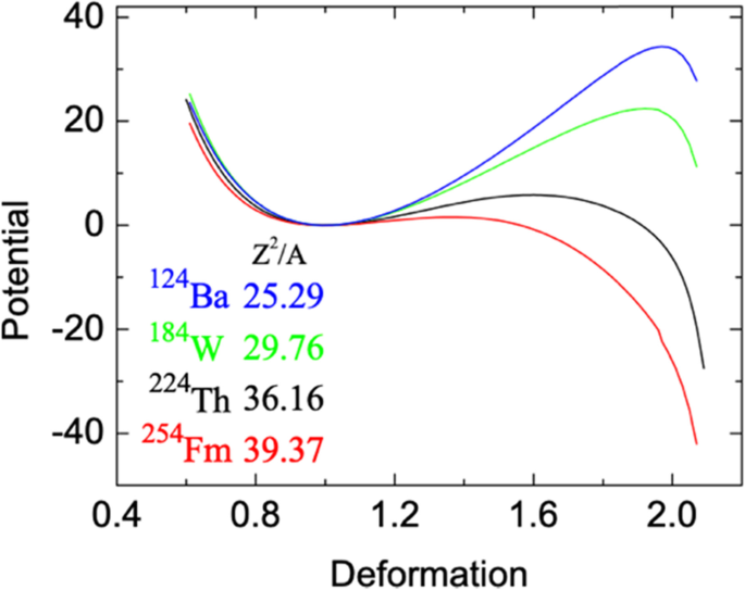
Liquid drop model potential as a function of deformation for different combinations of A and Z. Values of Z2/A are indicated. The deformation of 1 corresponds to the spherical shape. The figure is adapted from [25]
Figure 2a illustrates the effect of shell correction in the LDM potential along the primary fission coordinate, i.e. elongation. Subsequently, to explain the observed double-humped structure of FFMD, M\(\ddot{\mathrm{o}}\)ller and Nix [26] extended the work of Strutinsky by introducing the mass-asymmetry coordinate as an additional shape degree of freedom. The shell-corrected two-dimensional potential energy surface (PES) is depicted in Fig. 2b, and it indicates the preference for an asymmetric mass splitting.
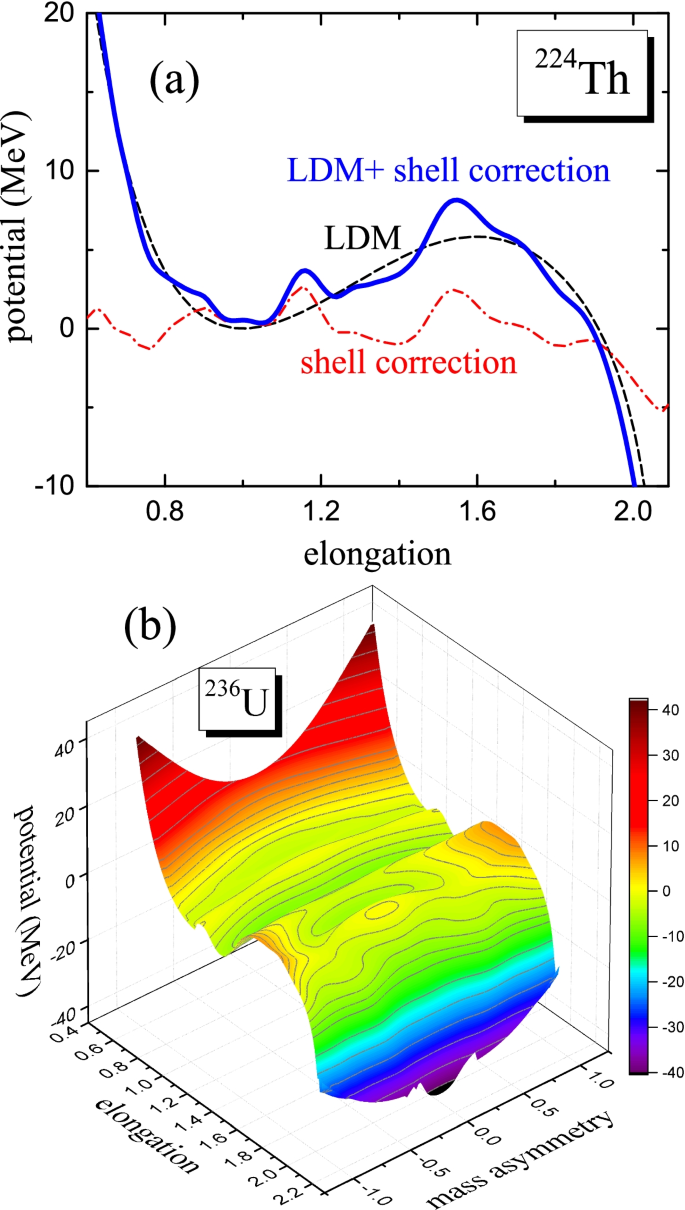
a Potential profile (solid line) of 224Th after adding shell correction (dash-dotted line) to the liquid drop potential (dashed line). b Two-dimensional potential energy surface of 236U obtained within the mac-mic description
The latest major development in the mac-mic potential was carried out by M\(\ddot{\mathrm{o}}\)ller et al. in 2001 [27]. In the PES calculation, they incorporated five independent collective degrees of freedom namely the elongation, mass-asymmetry, radius of the neck formed between the nascent fragments, and deformations of the nascent fragments. Appropriate fission dynamics [28] on a five-dimensional potential energy hypersurface can successfully reproduce the measured FFMDs for a good number of nuclei with stable or near-stable mass and atomic numbers. Furthermore, in a recent study [29], global calculations of FFMDs are attempted within the mac-mic framework. Apart from these, different versions (either the potential parameters or the collective coordinates are different) of mac-mic potentials [30,31,32] are often used to analyse measured fission data such as fission yields and their angular distributions, different cross-sections, and fission timescales. Although mac-mic models can precisely predict the fission observables for nuclei lying in and around the β-stable region, their extrapolation to the terra incognita may appear to happen to be inappropriate. For example, the recent FFMD model [29] overpredicts the measured fragment-mass width for 258Fm. In this respect, let me reiterate that the present versions of mac-mic model may suffer from large model-dependent uncertainties when applied to an unknown domain of nuclei. Although model-dependent uncertainties are present even in fully microscopic approaches, the predictive power of such models can be systematically improved with suitable theoretical tools. For example, as discussed in the following section, current microscopic theories focus on superior predictive power with a quantified theoretical uncertainty in the calculated potential energy [7]. It allows one to optimize the model parameters in order to reduce the uncertainty.
The first milestone of fission theory was laid by Niels Bohr and John A. Wheeler in 1940 [33]. They conjectured that a certain class of nuclear reactions takes place in two consecutive steps. First, an excited compound nucleus (CN) is formed with a comparatively long lifetime such that the excitation energy is uniformly distributed among all the degrees of freedom. Then, the equilibrated CN disintegrates to a less excited system by emitting light particles (mainly neutron, proton, and α) or γ-ray. On the other hand, it may break apart via fission where a reasonable part of the excitation energy transforms into the deformation potential and the collective kinetic energy. In addition to the hypothesis of thermal equilibrium, they further proposed the transition state theory where fission-decay probability (the number of events that decays via fission out of the total number of CN formed) is estimated by using the concept of statistical phase space counting. In this model, the number of fission events is assumed to be equal to the number of compound nuclei formed at the transition state: The nuclear configuration at the saddle point of the compound nuclear potential.
Subsequently, Peter Fong extended the idea of statistical equilibration in the calculation of FFMD [34]. He argued that the fission mode should not be determined at the saddle point since the decay actually occurs at a much later stage where the decaying CN attains a shape such that it is ready to come apart. This configuration is known as the scission configuration. Furthermore, different scission configurations can be possible depending on the magnitude of mass asymmetry between the probable fragments. The number of quantum states for each scission configuration gives the relative probability of the corresponding fragmentation mode. This methodology is, in general, known as the scission point model (SPM). It is quite popular as the calculations are time-efficient in comparison to a microscopic dynamical framework, and, also, it is easy to implement in a numerical program. More importantly, SPM can properly handle the excitation energy of a fragmenting nucleus, where quantum states for the scission configuration can be enumerated from the self-consistent energy density functional (EDF) formalism [35]. Over the years, SPM has undergone several refinements, and, therefore, different versions of this model are available. Recently, SPM is used to predict FFMDs of astrophysical nuclei with a broader aim to implement it in a r-process network calculation [36]. Despite several advantages, the application of SPM is limited since the pre-scission dynamics cannot be accounted for within such a static formalism.
For a long time, static models were quite successful in explaining the experimental fission data. Now, let me briefly explain how the scenario changed after 1980s when the acceleration of heavy ions became feasible in laboratories. Measurements in heavy-ion-induced reactions revealed enhancement in the neutron multiplicities as compared to statistical model predictions [37]. This experimental finding was accompanied by theoretical investigations based on the classical stochastic dynamics that usually predicts reduced fission probabilities due to dissipative effects. In addition, experimental evidences from other probes like charge-particle multiplicities, γ-ray from giant dipole resonance, fission-fragments’ kinetic energy distribution, and evaporation residue cross-section also suggested that the fission dynamics is dissipative in nature. Theoretically, justification in favour of the viscous effects during fission was first raised by Kramers’ long back in 1940 [38]. He derived an analytical expression for fission width by implementing several simplifying assumptions in the Fokker-Planck equation. An elaborate description of the Fokker-Planck dynamics and subsequent derivation of the Kramers’ equation can be found in Ref. [39]. Currently, Kramers’ theory is routinely used to invoke energy dissipation mechanisms in statistical model calculations [40].
The origin of nuclear dissipation can be understood within the adiabatic approximation [25]: τeq ≪ τcoll, where τeq is the equilibration time of the intrinsic degrees of freedom and τcoll is the typical time scale of collective motions, i.e., the time over which the collective coordinates (usually nuclear shape parameters are used as collective coordinates, see next section) change significantly. Under this assumption, the total Hamiltonian Htotal of a fissioning nucleus can be decomposed as,
where Hcoll consists of the collective kinetic energy and the driving potential due to change in deformation, Hintr is the intrinsic energy corresponding to the random motion of nucleons, and Hcoup is the interaction between the collective and random degrees of freedom. Since Hintr contains almost the entire Htotal, it remains unperturbed by Hcoup. Therefore, the intrinsic excitation energy is often considered to form a heat reservoir/bath. Furthermore, within the canonical thermodynamical model for non-interacting Fermions, we assign a particular temperature to the heat bath by following the energy conservation principle. Here, Hcoup causes dissipative energy transfer between Hcoll and Hintr through the fluctuation-dissipation mechanism. The above scenario is illustrated schematically in Fig. 3. The fluctuating force exerted by the heat bath helps the system (collective coordinate) to overcome the potential barrier, and, as an opposing effect, dissipation transfers the collective kinetic energy to the heat bath.
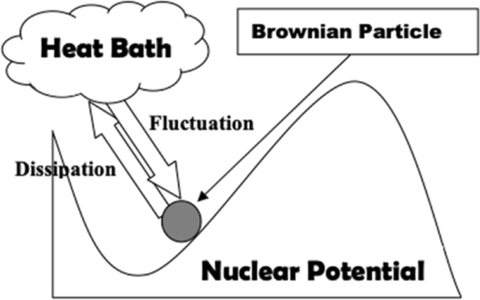
A schematic diagram of the dissipative dynamical model for fission. The figure is adapted from [25].
The nature of the dissipation mechanism is a long-debated issue in nuclear collective dynamics. Two available choices for nuclear dissipation/friction are the one-body dissipation, which is also known as the wall friction (WF) [41], and the hydrodynamical two-body dissipation arising from two-body collisions among the nucleons. The one-body mechanism can be described by combining the nuclear mean-field approximation with the classical treatment of an ideal gas. Here, nucleons are assumed to undergo collisions with the moving nuclear surface, and thereby damp the surface motion [41]. The irreversibility criterion of dissipation appears after taking the time average of the transferred momentum. Equivalent quantum description for the one-body dissipation was also prescribed [42]. In the past century, extensive studies were performed to identify the appropriate choice for dissipation model in low energy nuclear phenomena like fission, and it was concluded that the hydrodynamical two-body viscosity cannot give a consistent explanation of both neutron multiplicity and fission fragment kinetic energy distribution [43]. On the other hand, these observables indeed support the one-body mechanism. Similarly, the studies of macroscopic nuclear dynamics, such as those encountered in a low-energy collision of two heavy nuclei, indicate that the one-body dissipation is the most important mechanism for the damping of collective kinetic energy.
The WF formula was originally derived for a fully chaotic classical gas. Hence, it requires finer corrections while applying to nuclear dynamics. One major difference between a classical gas and a nucleus is that the motion of nucleons is not fully chaotic during the collective dynamics, since n-n collisions are rare at excitation energies much below the Fermi energy. The chaos weighted wall friction (CWWF) is suggested [44] to resolve this issue, and it predicts the fission observables better than the original WF [45]. In spite of numerous theoretical and experimental investigations, an accurate determination of nuclear dissipation strength is still remaining as an open problem. Along this direction, shell corrections are incorporated [46] in the transport coefficients like inertia and friction, and these modified inputs can provide good agreement with the measured data without any fitting parameter. However, a global survey with these shell-corrected transport coefficients is still needed. In addition, a fully microscopic calculation of nuclear dissipation from effective n-n interactions is yet to be pursued [1]. Therefore, the dissipation strength is often used as a free parameter in analysing fission measurements.
The stochastic Langevin dynamics and the Fokker-Plank diffusion equation are the two alternatives that can be used to simulate the shape evolution of an excited nucleus. The Langevin dynamical framework was first applied to fission by Y. Abe in 1986 [47]. This method directly deals with the time evolution of nuclear collective coordinate(s). Therefore, it is apparently more intuitive than the Fokker-Planck equation that assumes a distribution function for the collective coordinates. In one-dimensional Langevin dynamics, the equations of motion for the dynamical (collective) coordinate are written as [25]
where q and p represent the collective coordinate and the conjugate momentum, respectively. \(\mathcal{M}\) is the collective inertia which may be shape-dependent, and V is the driving potential generated from nuclear interactions. In the second equation, the terms outside the parenthesis are (1) a slowly varying part which describes the average effect of heat bath on the particle, and is called the friction force (βp); (2) the rapidly fluctuating part which has no specific functional dependence on t, and it is called the stochastic (random) force (Γ(t)). Usually, the time correlations of Γ(t) are assumed to be the same as that of the white noise: 〈Γ(t)〉 = 0, 〈Γ(t)Γ(t′)〉 = g2δ(t − t′); g being the strength of the random force. The dissipation strength β is related to g through the Einstein’s fluctuation-dissipation theorem [48]: g2 = βT.Due to the random force, different Langevin trajectories originating from the same initial configuration may end up at different scission point. Thus, a distribution of scission configurations is generated when an ensemble of events is sampled on a multidimensional PES. A typical Langevin trajectory calculated on the two-dimensional configuration space of elongation and mass-asymmetry is shown in Fig. 4. This trajectory is obtained with the WF and the hydrodynamic collective inertia, which is frequently used in mac-mic models. Langevin dynamical calculations are widely used [30,31,32, 49] to investigate heavy-ion induced fission at relatively higher energies, where large angular momentum and excitation energy are generated. One major advantage of the Langevin framework is that the model is easy to implement numerically in a computer code. Also, it incorporates the dynamical effects like dissipation in a proper way. In fact, Randrup et.al. showed [28] that the fission dynamics is overdamped in nature to a certain extent, and, hence, the effects due to collective inertia can be neglected. This idea guides to the Brownian shape motion (BSM) approach [28] that successfully reproduces the FFMDs for heavy nuclei above A~220. Although the BSM model incorporates the dynamical effects, the interplay between the dynamics and the thermalization process is yet to be explained in a more comprehensive manner [1, 50].
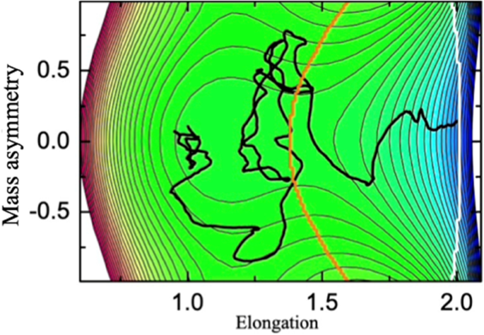
A typical fissioning Langevin trajectory on the LDM potential energy surface of 224Th calculated for compound nuclear angular momentum and temperature of 60ℏ and 2MeV, respectively. The orange and white lines are the saddle ridge and scission line, respectively. The figure is adapted from [25]
In spite of several benefits, the Langevin approach may not be appropriate for low energy fission, where quantum correlations are important. Moreover, the collective dynamics near scission may become fast enough so that the adiabaticity condition is violated [51]. Also, in the context of practical applications, available Langevin frameworks are usually composed of phenomenological mac-mic potentials, which may lack the structural features of very massive elements and of r-process nuclei.
The previous section establishes that a complete microscopic theory is a prerequisite for scrutinizing fission dynamics. As I mentioned before, we require a quantum many-body formalism to achieve this goal. However, an unified microscopic framework that accounts for all the characteristics of fission dynamics is still missing. Therefore, different theoretical formalisms are used in practice, depending on their applicability and inherent features. For example, almost all the fission models, except the time-dependent density functional theory (TDDFT) [52,53,54,55], assume the adiabaticity approximation. Therefore, in those models, a static PES is first generated and then the time evolution is followed with a suitable dynamical framework. On the other hand, TDDFT is more general in a sense that the time evolution is studied without a priori assumption on the timescale of collective motion. Moreover, dissipative effects can be best accounted for within TDDFT. Albeit very promising, the current implementations of TDDFT handle several important aspects of nuclear structure (centre of mass, nuclear superfluidity) rather crudely and cannot always properly describe collective correlations [52]. In addition, such calculations can only simulate the average fission trajectory: reconstructing statistical distributions in TDDFT requires the inclusion of density fluctuations, which is restricted by the current computational capabilities [56]. It is worth noting that the relativistic density functional theory [57] can also be applied to study nuclear dynamics in heavy nuclei. Relativistic TDDFT is recently used [58] to study light-ion reactions. This framework can be generalized for fission dynamics. In the rest of this article, I will elaborate on the different aspects of microscopic models and their applications in fission dynamics. Detailed reviews on this topic can also be found in Refs [7, 54, 59, 60].
The first step towards a microscopic calculation of fission dynamics within the adiabatic approximation is the determination of static PES. Phenomenological shell models that describe the motion of independent nucleons in a mean-field potential, fail [61] to reproduce the total energy of a nucleus. Also, a proper shell model calculation [62] with residual interactions requires a very large valance space to estimate the energy for heavy and deformed nuclei. To this end, nuclear DFT provides an ideal platform, where potential energy is calculated form effective n-n interactions in a self-consistent manner. In this approach, Hartree-Fock-Bogoliubov (HFB) equation [61] is solved by constraining different mass multipole moments. These moments also serve the purpose of dynamical coordinates. The long-range mean field part of the HFB energy is obtained from either a relativistic or a non-relativistic version of EDFs. Two well-known families of non-relativistic n-n interactions are the finite-range Gogny force and the zero-range Skyrme force. Since the Skyrme force comprises of only local interactions, corresponding EDFs are easy to implement in realistic calculations. Also, in the case of Skyrme EDFs, pairing fields are determined independently (not true for UNEDF). Recent developments in the Skyrme functionals are performed within the UNEDF project [63], and one of its variants, UNEDF1HFB [64], is successfully applied to fission dynamics [65,66,67]. Although the DFT framework can be derived for a standard two-body interaction, the latest Skyrme EDFs contain terms with fractional powers of the one-body density. These cannot be associated to a two- or three-body interaction.
With the present-day computational power, HFB Hamiltonian can be diagonalized without invoking any symmetry restrictions on the basis states. One major advantage of DFT based calculations is the following. Here, we need to constrain only those multipole moments which are pertinent to the required observables, and all the other moments are optimized through the self-consistency (energy minimization) criterion. Therefore, potential energy obtained from the DFT calculations is, in principle, more accurate. In practice, discontinuities may appear in DFT potential as a result of a limited number of multipole constraints [68]. This problem can be circumvented with a proper check on the unconstrained higher-order multipole moments. As a representative example of DFT potential, the PES of 258Fm is presented in Fig. 5 along with the symmetric and a typical asymmetric fission pathways. Different self-consistent shapes on these two paths are also shown. Although only the axial quadrupole (Q20) and octupole (Q30) moments are constrained to generate the PES, shapes at large Q20 may develop large hexadecapole moment (Q40) as an outcome of the energy minimization process.
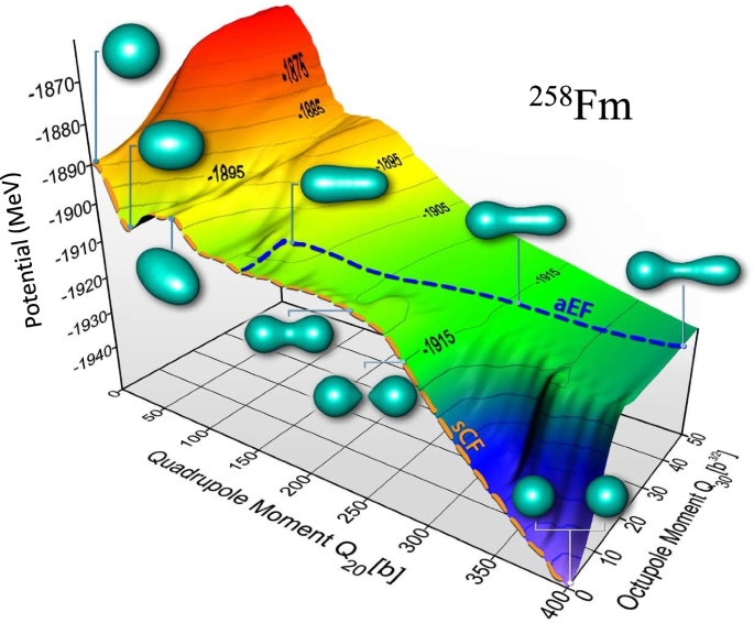
Potential energy surface of 258Fm calculated along quadrupole (Q20) and octupole (Q30) mass moments. Symmetric compact fission (sCF) and asymmetric elongated fission (aEF) paths are drawn using dotted lines. Nuclear shapes along these paths are shown for specific values of Q20 and Q30 as indicated. The figure adapted from (https://people.nscl.msu.edu/~witek/fission/fission.html)
As I mentioned, quantification of uncertainties is an important aspect to assess the predictive power of a theoretical model. It can be implemented in DFT based calculations. On an evolutionary path of nuclear DFT, different parametrizations for n-n interactions are recommended to fine-tune different classes of nuclear observables. For example, the PES in Fig. 5 is calculated for the SkM* parametrization of the Skyrme EDF, which is optimized to predict large-amplitude collective dynamics. Hence, it is widely used in fission studies. In contrast, a relatively smoother potential profile with a lower fission barrier height (see Fig. 6) is predicted by the advanced UNEDF1 functionals [69]. Although this overall reduction in the potential barrier may be attributed to the proper accounting of the particle-particle correlations in UNEDF1, the model parameters in both the EDFs cannot be determined uniquely if one attempts a global optimization over a large span of known nuclei. To this end, analysis of theoretical statistical uncertainties in EDF parameters is crucial, and it can be performed with the help of the Bayesian inference methods [69]. One effort along this direction is demonstrated in Fig. 6, where the grey band signifies the variation in potential energy corresponding to the 90% confidence interval in the EDF model parameters.
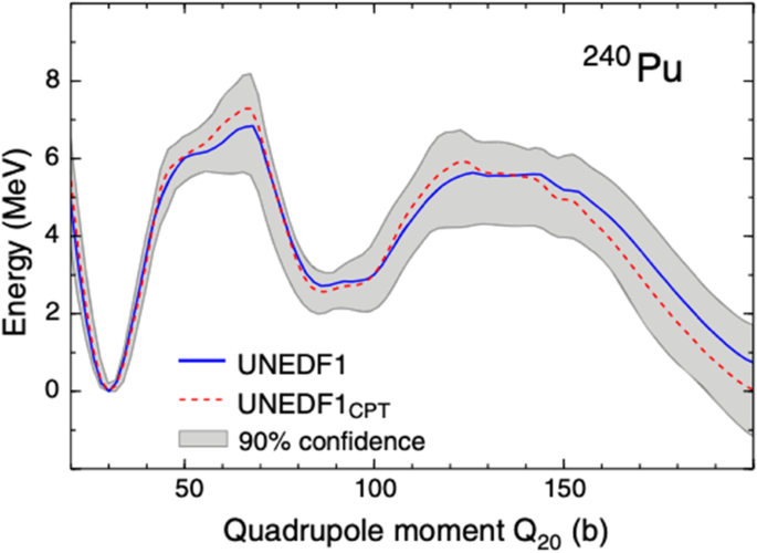
Potential energy profile for 240Pu calculated with UNEDF1 (solid line) and UNEDF1CPT (dashed line, suffix CPT indicates that the parameters are optimized on a data set that also includes masses measured at the Canadian Penning Trap) EDF. Gray area is the 90% confidence interval of the potential profile. The figure is adapted from [69]
A similar comparison for different kinds of EDF is demonstrated in Fig. 7. Evidently, the two-dimensional PES from UNEDF1HFB is comparatively flat with respect to the results corresponding to SkM* and D1S functionals [65]. In spite of this diversity, I would emphasise that the overall structures of these PESs are very similar. It elucidates the robustness of model predictions in the domain of DFT calculations.
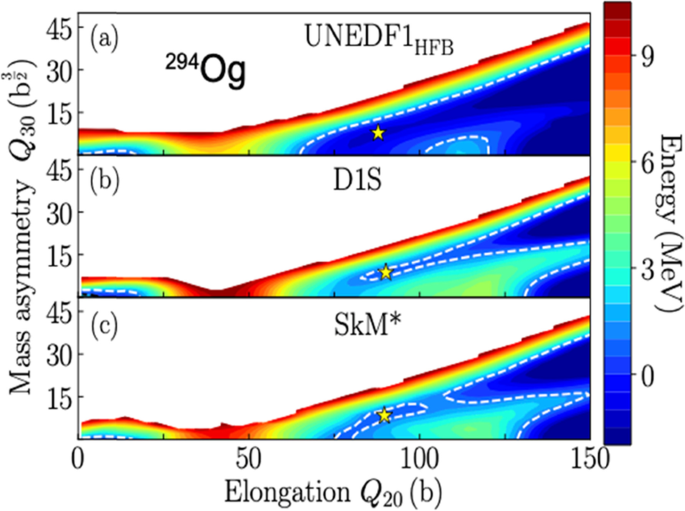
2D Potential energy surface of superheavy element 294Og, calculated with different density functionals as mentioned. The ground state energy Eg. s. is normalized to zero. Dotted lines indicate E0 − Eg. s. = 1 MeV. The local energy minima at large deformations are marked by stars. The figure is adapted from [65]
The evolution of a nuclear system in SF can be viewed as a dynamical two-step process [56]. The first phase involves quantum tunnelling through a multidimensional potential barrier. Dynamics of this process is adiabatic in nature as the SF lifetime is, in general, large compared to intrinsic nucleonic motions. Moreover, it is governed by the collective inertia. The tunnelling phase ends at the outer turning point (or hypersurface in case of a multidimensional configuration space). Beyond the outer turning point(s), the deformed nucleus propagates in a classically allowed region before reaching the scission configuration. Collective motion in this second phase has a dissipative character and, therefore, the corresponding microscopic description involves potential, inertial, and dissipative aspects [56]. Both the steps are illustrated in Fig. 8 for the one-dimensional potential profile of 240Pu.

Potential energy of 240Pu calculated along the most probable fission path. In the classically forbidden region (marked WKB; between the inner turning point “in” and outer turning point “out”), the collective action is minimized to determine the half-life. In between the outer turning point and scission, the evolution of the system can be described by stochastic Langevin dynamics. E0 is the quantum zero-point energy at the ground state configuration. The x-axis gives the quadrupole moment of the fissioning nucleus and it is equivalent to the elongation coordinate used in mac-mic models. The figure is adapted from [56]
The tunnelling phase can be described by instanton methods that account for some form of dissipation between collective and intrinsic degrees of freedom [70]. However, the practical application of this imaginary-time approach with realistic PES faces numerous difficulties [71]. Consequently, calculations of tunnelling probabilities are mainly based on the semiclassical WKB approximation that depends sensitively on the interplay between the static nuclear potential energy and the collective inertia. Precisely, the SF half-life can be written as T1/2 = ln 2/(nP) [72], where n is the number of assaults on the fission barrier per unit time. P is the WKB penetration probability. It is calculated from the relation, P = 1/(1 + e2S), where S is the action integral given by [72],
In the above equation, integration is performed along various paths on the PES. \(\mathcal{M}(q)\) and V(q) are effective inertia and potential energy, respectively, along the fission path. The SF probability corresponds to the minimum of the action integral S. The fission path is decided from this minimum action criterion. Two different numerical techniques are available to extract the minimum action path. One of them is known as the dynamical programming method (DPM) [59] where the whole configuration space is divided into a mesh, and then the fission coordinate is propagated from one layer to the next one by tracing the overall minimum in the action integral. On the other hand, in the Ritz method (RM) [72], the fission path is expanded in terms of a Fourier series expansion. The coefficients of the expansion are then optimized to extract the minimum action. Although the second method is computationally faster, DPM is easy to implement on a complicated topology of the configuration space. Advanced studies are in progress to develop a more efficient action minimization technique.
The choice of the static potential is an important input for the calculation of the action integral. Especially, delicate structural changes in V(q) (Eq. 2) can strongly impact P because of its exponential dependence on S. Therefore, for unstable systems like SHE and for exotic nuclei, it is desirable to extract V(q) from a microscopic theory instead of the LDM based calculations. For example, the state-of-the-art computational framework based on the self-consistent symmetry-unrestricted DFT is applied in Refs. [16, 73] to compare the SF half-life (TSF) with the α-decay half-life (Tα) for a wide range of SHE (Fig. 9).
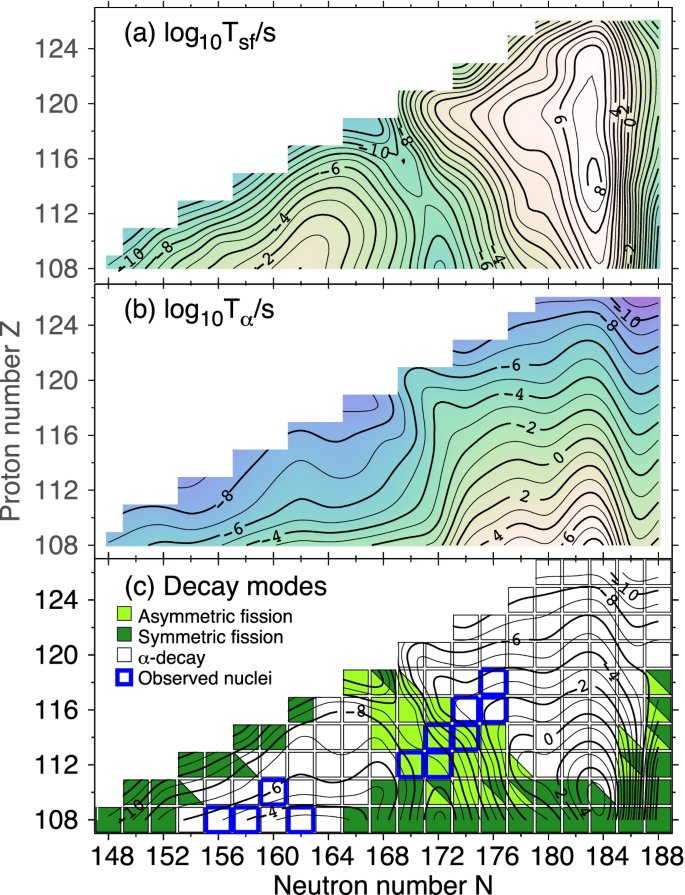
a Inner fission barrier heights (in MeV). b SF half-lives log10TSF (in seconds). c α-decay half-lives log10Tα(in seconds). d Dominant decay modes. If two modes compete, this is marked by coexisting triangles. The figure is adapted from [16]
Moreover, as shown in Fig. 9, the fission decay mode (mass symmetric or asymmetric) is also determined for the subset of nuclei which predominantly decay via SF. Interestingly, as predicted in [16], the short-lived super-heavy isotopes 280Hs, 284Fl, and 284Og, which are candidates for SF decay, form a narrow corridor in between the regions of SHE synthesized in cold-fusion and hot-fusion reactions.
Apart from the potential energy, Eq. (2) is very sensitive to the collective inertia. For a long time, perturbative cranking inertia was the most suitable choice for microscopic inertia. Then, Baran et.al. show [74] that the nonperturbative cranking inertial contains sharp variations that are absent in the perturbative version. Furthermore, in a separate study [75], it is demonstrated that these rapid variations are associated to nuclear structural changes triggered by the crossing of single-particle levels near the Fermi surface. Also, the two-dimensional SF paths are calculated with perturbative and nonperturbative cranking inertia. This work [75] predicts that the dynamic least-action pathway becomes strongly triaxial when nonperturbative inertia is used, and it approaches the static fission valley defined from the potential minima. In contrast, as illustrated in Fig. 10, perturbative cranking inertia tensor restores the axial symmetry along the path to fission. This can be explained [75] as an artefact of the perturbative approximation. Also, Fig. 10 confirms that the results from the two different path minimization techniques (DPM and RM) are consistent. Similar calculation [76] with relativistic EDFs reaffirmed the above dependence of the fission pathway on the choice of collective inertia. In a very recent work [77], cranking inertia is calculated by incorporating the effects due to time-odd densities. This is a major accomplishment that may substantially modify the SF half-life.
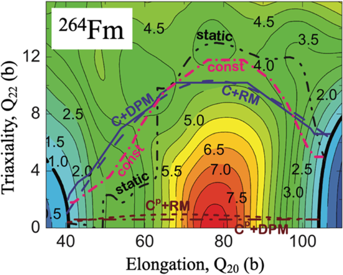
Dynamic paths for spontaneous fission of 264Fm, calculated for the nonperturbative (“C+DPM”, “C+RM”) and perturbative (“Cp+DPM”, “Cp+RM”) cranking inertia using DMP and RM techniques. The static pathway (“static”) and that corresponding to a constant inertia (“const”) are also shown. The figure is adapted from [75]
It is also noticed [78] that the nuclear pairing correlations may strongly impact the SF path. Pairing interaction or the nuclear superfluidity tends to make the collective dynamics more adiabatic by suppressing the configuration changes prompted by level crossings. Competition between these two opposing effects has a profound impact on SF lifetime [78]. Whereas nonperturbative inertia enhances the SF half-life of 264Fm by two orders of magnitude [77], dynamical pairing reduces it by four orders. Therefore, it is proposed in Ref. [78] that, for precise estimation of SF lifetime, nuclear pairing must be incorporated as an additional dynamical coordinate in the calculation of the fission pathway.
Now, let me focus on the calculation of SF yields. Static approaches like different variants of SPM can be used to calculate SF yields. However, such calculations lack all dynamical effects arising due to the evolution of the system in the configuration space. On the other hand, the application of quantum dynamics like the time-dependent generator coordinate method (TDGCM) (described in the next section) is not feasible as SF dynamics may involve very large dynamical time. Recently, a TDDFT framework is designed [79] for calculating SF yields. However, such calculations have computational restrictions. An elaborate discussion on this model is presented in Sec. 4.4. Also, a hybrid model is developed [56] to calculate the SF yields by following the post-tunnelling dynamics with the stochastic Langevin equations. This scheme has already been portrayed in Fig. 8. The calculated FFMD in Ref. [56] ensures that the PES is the most important ingredient when it comes to the peaks of the yield distributions. This finding agrees with other DFT based studies [80,81,82], also concluding that the topology of the PES in the pre-scission region is a decisive factor for the most probable mass splitting. On the other hand, as demonstrated in Ref. [56], both the dissipative collective dynamics and the collective inertia are essential when it comes to the shape of the yield distributions. Moreover, the SF yield distributions from the hybrid model are found [56] to be fairly robust with respect to the details of dissipative aspects of the model.
The hybrid model is further employed [65] to predict the fission modes of the superheavy 294Og. According to theory, superheavy nuclei predominantly decay via highly asymmetric fission mode [83], also known as cluster decay, where the heavy fragment prefers to be doubly magic 208Pb. Experimental search for the cluster emission has been initiated [84]. However, limitations appear as SHE are produced in laboratories at non-zero excitation energies [85], where the shell effect completely melts down. Calculations in Ref. [65] predict that the dominant spontaneous fission mode of 294Og will be centred around doubly magic 208Pb and magic 86Kr. Also, Ref. [65] shows that this prediction is almost independent of the choice of input parameters such as energy density functional, collective inertia, and dissipation tensor. In particular, I emphasise that the difference in barrier heights, as shown in Fig. 7, does not affect the fission yields. For completeness, calculated yields of 294Og are plotted here in Fig. 11 on the N-Z plane of known nuclei. I conclude this section by stating that, although SF lifetime is strongly influenced by factors like the choice of EDF and collective inertia, associated yield distributions are almost insensitive to these finer details.
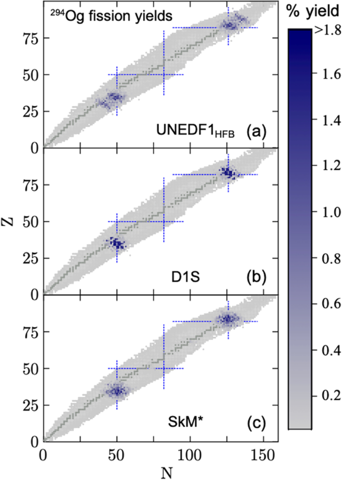
Fission fragment distributions for 294Og calculated with the three EDFs using the hybrid (WKB+Langevin) model as discussed in the text. Known isotopes are marked in grey. Magic numbers 50, 82, and 126 are indicated by dotted lines. The figure is adapted from [60]
The time-dependent generator coordinate method (TDGCM) is a microscopic framework to study large-amplitude dynamics within the adiabatic approximation [61, 86,87,88]. In this model, the many-body state ∣ψ(t)⟩ of a fissioning system is expanded in terms of the so-called generating functions {| ϕq⟩} as,
where the continuous variables q ≡ (q1, q2, …qN) are the dynamical (collective) coordinates and the coefficient f(q, t) is called the weight function. When the variational principle is applied to the total energy \(\left\langle \psi (t)\right.\mid {\hat{H}}_{\mathrm{total}}\mid \left.\psi (t)\right\rangle\) with the variations in q, it yields the time-dependent Hill-Wheeler equation for f(q, t) that governs the evolution of the fissioning nucleus. This equation can be written as
An exact solution of Eq. (4) is too complicated, and, therefore, the Gaussian overlap approximation (GOA) is often used, where the overlap between two generator states ⟨ϕq| ϕq′⟩ is assumed to be a Gaussian function of (q − q′). Equation (4) then reduces to a local time-dependent Schr\(\ddot{\mathrm{o}}\)dinger like the equation for the collective Hamiltonian \({\hat{H}}_{\mathrm{coll}}\left(\boldsymbol{q}\right)\) [88],
Here \({\hat{H}}_{\mathrm{coll}}\left(\boldsymbol{q}\right)\) contains the static potential V(q) and the collective inertia \(\mathcal{M}\left(\boldsymbol{q}\right)\). g(q, t) is related to the weight function f(q, t). An initial collective wave packet g(q, t) is propagated with Eq. (5). Eventually, the flux of g(q, t) at scission gives the yield distributions. Two mentionable drawbacks of this method are (1) dissipative effects are not accounted and (2) limitation appears due to the presence of discontinuities in the two-dimensional manifold of generator states [86].
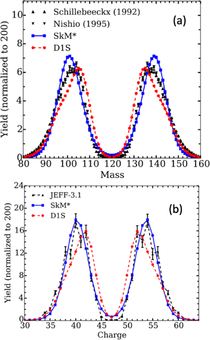
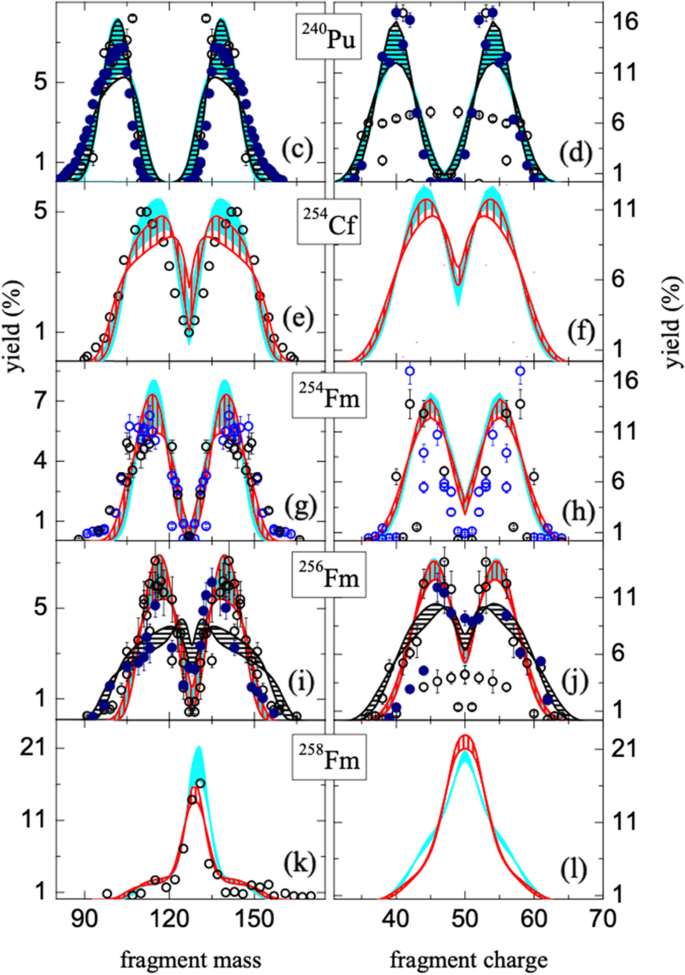
The TDGCM+GOA [61, 88] formalism provides the microscopic alternative to the classical Langevin dynamics. In principle, it maintains the quantum correlations which are essential for low-energy fission. The method is regularly used to study fission fragment yields and their total kinetic energy in the case of thermal fission [86, 89,90,91]. For example, fragment mass and charge distributions for the thermal fission of 239Pu are demonstrated in Fig. 12. Furthermore, TDGCM can qualitatively describe [92] the asymmetric to symmetric transition in the fission yield distributions of neutron-rich fermium isotopes. This makes it a promising tool to investigate the evolution of fissioning nuclei away from the valley of stability. Besides induced fission, TDGCM can also be employed to study spontaneous fission [93].
A non-adiabatic microscopic theory to study fission dynamics is the time-dependent density functional theory (TDDFT) [53,54,55]. Originally, this formalism was developed with the help of the time-dependent Hartree-Fock (TDHF) equation [96]. It was first proposed by Dirac in 1930 [97]. For several decades, the application of TDHF was restricted to small amplitude dynamics due to limitations in the computational resources. Then, in 1976, TDHF was first used to study large amplitude dynamics in the nuclear matter [98, 99]. Subsequently, it became a powerful tool to investigate varieties of dynamical phenomena occurring at low-energy nuclear collisions [100]. Similar to the static DFT calculations, both relativistic and non-relativistic versions of TDHF formalism exist.
Apart from nuclear collisions, a principal application of TDHF is to study collective vibrations [101,102,103]. In the linear regime, TDHF leads to fully self-consistent random phase approximation (RPA), for which often additional approximations are employed. Response from the giant dipole resonance (GDR) of a nucleus can be calculated microscopically by employing different variants of RPA and quasiparticle-RPA (QRPA). Finite-temperature QRPA was also prescribed to study GDR build on an excited state. In addition, TDHF can be used to investigate non-linearities of nuclear vibrations [104].
The TDHF framework has gone through several refinements in recent times. I would like to mention a few of them. (1) The effective nucleus–nucleus potentials can be extracted with and without dynamical effects. This can be achieved either by employing the frozen HF method [105] or by constraining the density. The second technique is known as the density-constrained TDHF (DC-TDHF) method [106]. (2) The fission fragments can be identified by using the particle number projection technique [107]. (3) The absence of fluctuations in physical observables is a major limitation in TDHF theory. Initiatives [108,109,110] are being taken to incorporate fluctuations of one-body observables by using the Balian–Vénéroni variational principle. (4) In an advanced version (known as TDHF+BCS), dynamical pairing correlations are incorporated [53, 111] in TDHF following the Bardeen–Cooper–Schrieffer (BCS) prescription. (5) The nucleon localization function (NLF) [112] provides superior structural information compared to the scalar density. The time-dependent NLFs are evaluated in a work [113] to reveal the structure of pre-compound states in nuclear reactions involving light and medium-mass ions. The NLFs for the 16O+16O collision are plotted in Fig. 13 as a representative example from this work. It is clearly visible that the α-12C-12C-α substructure appeared for the three impact parameters chosen in this work. Also, while the colliding system conserved the axial symmetry for the central collision, a marginal shift in the α clusters toward the direction of rotation can be noticed for non-central collisions.
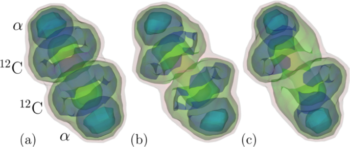
The NLFs for α-12C-12C-α structure formed at t = 300 fm/c in 16O + 16O collision at Ecm = 20 MeV for three values of the impact parameter: b = 0 fm (a), b = 2 fm (b), and b = 4 fm (c). The colour scale is 0.55 light red, 0.65 green, 0.75 blue, and 0.85 cyan. The figure is adapted from [113]
In the case of fission decay, it is experimentally observed that the fission fragments of actinide nuclei peak around atomic numbers 52 ≤ Z ≤ 56, indicating the presence of finer effects apart from the Z = 50 spherical shell closer. In a superfluid TDHF calculation [53], it is demonstrated that the heavy fission fragments of actinides prefer to have 52–56 protons. This is in accordance with the large gap in single-particle energies triggered by the octupole deformation of the nascent fission fragments [114]. In another calculation [115], fission modes of sub-lead nuclei are investigated by using the TDHF formalism, and it confirms that the mechanism responsible for asymmetric fission in the sub-lead nuclei is the same as in actinide nuclei. Precisely, the quantum shell effects that stabilize the pear shape of a fission fragments, also explain the origin of asymmetric fission in both the mass regions. As shown in Fig. 14, the most probable fission path of 180Hg supports the above-mentioned fact. Precisely, the asymmetric pathway produces 100Ru and 80Kr as the most probable fragments. Here 100Ru corresponds to the deformed shell gap at neutron number 56.
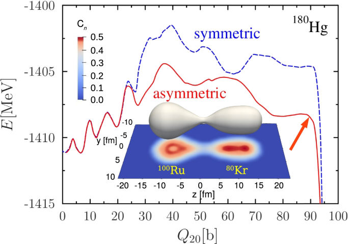
Potential energy profile along the symmetric (dashed line) and an asymmetric (solid line) fission pathway of 180Hg. Equal density surface at half-saturation density of 0.08 particles/fm−3 and the projection of neutron NLF are shown for a quadrupole shape just before scission in the asymmetric fission valley (marked with the red arrow). The figure is adapted from [115]
To mimic fluctuations in the TDHF framework a new technique is proposed in Ref. [79]. In this approach, density fluctuations are assumed to prepare an ensemble of different configurations. Specifically, the method is applied to SF and, therefore, the density ensemble is constructed outside the barrier region and the subsequent propagation is followed with the standard TDHF+BCS theory. The total kinetic energy (TKE) distribution and the fragment mass distribution for SF of 258Fm are calculated [79] by employing this model. Figure 15 displays the comparison of the calculated distributions with experimental data. It reveals that, although there is a good overall agreement between the calculated results and the data, the width of the mass distribution is underestimated. The possible reason could be: The density fluctuations in [79] are restricted to somewhat smaller configuration space around the mass-symmetric deformation. However, a more exhaustive calculation would require huge computational efforts.
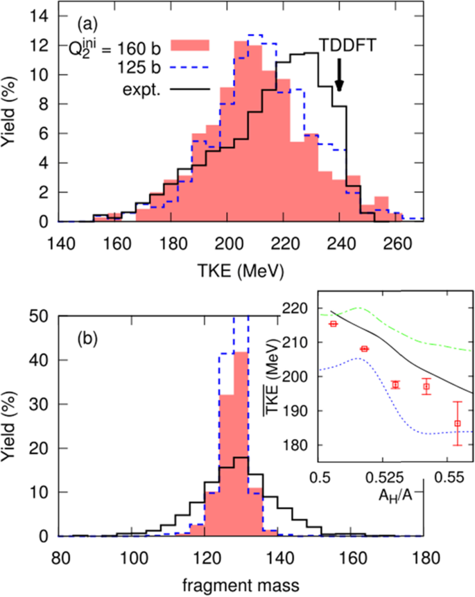
The TKE (a) and fragment mass (b) distributions obtained when an elongated (shaded areas) and compact (dashed lines) initial post-saddle deformations are considered. The solid lines are the experimental data [116]. In a, the arrow indicates the mean experimental TKE. In the inset of b, the correlation between the average TKE and heaviest fragment mass (red squares) is compared with results from the scission point model [117] (dotted and dot-dashed lines). 257Fm data [118] is shown by the solid line. The figure is adapted from [79]
Apart from the standard TDHF+BCS approach, a different version of TDDFT formalism is developed where the dynamical paring is incorporated more accurately [111]. The fission pathway of 240Pu is calculated in this study, and it is found that the pairing correlation plays a crucial role in deciding the collective timescales. Furthermore, the nature of the fission dynamics is speculated to be quite surprising as the overall collective propagation appears to be much slower even without invoking any dissipative effects. In a subsequent study [50] by the same group, the collective motion is predicted to be highly dissipative due to the presence of one-body dissipation. This finding supports the validity of using the overdamped Brownian shape motion approach.
The concept of NLF was first borrowed from atomic physics where NLF is used to characterize chemical bonds in electronic systems. In nuclear physics, NLF was originally used to identify the cluster formation in light nuclei [119]. NLF measures the probability of finding two nucleons with the same spin and isospin at the same spatial localization. As illustrated in references [120, 121], the clustering of nucleons inside a nucleus can be identified more accurately by NLFs instead of the scalar density distributions. It is because the topology of NLFs exhibit a pattern of concentric rings that reflect the internal shell structure, but such patterns are averaged out in the density distributions. The concept of NLF motivates [65, 67, 120,121,122] the idea of prefragments, i.e., localized clusters in a fissioning nucleus. The method of identifying these prefragments is described in Ref. [121] for a typical case of elongated 240Pu nucleus. Corresponding NLFs are sketched in Fig. 16. Evidently, the parts of NLFs for z ≥ zL and z ≤ zH contain ring-like patterns delineating the presence of localized nucleons inside the deformed 240Pu.
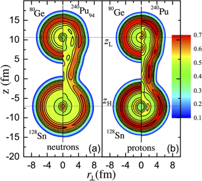
Neutron (a) and proton (b) NLFs in a deformed configuration on the fission path of 240Pu (right panels). NLFs of the localized prefragments, 80Ge and 128Sn, are compared (left panels). Vertical lines are symmetry axes. Maximum extensions of the NLFs along the radial coordinate r⊥(z) are marked with horizontal dotted lines: z = zL and z = zH. The figure is adapted from [121]
Once the prefragments are formed the elongated nucleus can be imagined as two well-formed prefragments connected by glue of nucleons in the neck. This proposition is further illustrated in Fig. 17. It shows the density distributions of neutron and proton prefragments, and the neck nucleons for an elongated configuration of 254Fm. It is observed [67] that two distinct prefragments develop and then separate well before scission is reached. This early formation of the prefragments is a manifestation of the freeze-out of single-particle energies along the fission pathway as the system tries to maintain its microscopic configuration to avoid level crossings. In fact, for actinide nuclei, one of the prefragments happens to be spherical due to the shell structure of the doubly magic 132Sn nucleus (see Fig. 17). These arguments motivate the work of Ref. [67], where a new framework is developed to calculate fission fragment yields. In this model, the distribution of the neck nucleons among the two prefragments is obtained by means of statistical probabilities. Importantly, this method provides an efficient alternative to microscopic approaches based on the evolution of the system in a space of collective coordinates all the way to scission. Therefore, it can be used to carry out global calculations of fission-fragment distributions across the r-process region. The new model is benchmarked in Ref. [67] by predicting the fission-fragment mass and charge distributions of some selected nuclei. These are shown in Fig. 18. In general, very good agreement with the experiment can be observed for both SF and thermal fission. Based on this benchmarking, it can also be inferred [67] that the proposed method is robust with respect to the choice of the EDF parameters because the SkM* and UNEDF1HFB results in Fig. 18 are quite close.
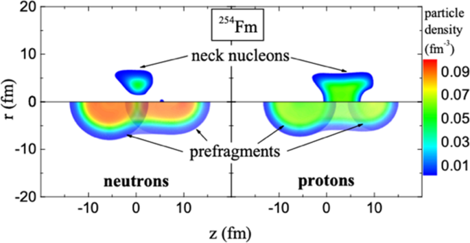
Density distributions of prefragments (bottom) and neck nucleons (top) obtained from DFT calculation with UNEDF1HFB. The figure is adapted from [62]
In this review, I elaborated on the theoretical modelling of fission dynamics. Attention has been given specifically to the microscopic theories based on effective n-n interactions. Due to enormous computational requirements and inherent restrictions, each of these models can only be applied in a limited domain of nuclear dynamics. A few of such examples are as follows. (1) The TDDFT framework is suitable for low energy dynamics where the time evolution can be described with a many-body wavefunction constructed in the Bogoliubov vacuum (or BCS ansatz). However, the influence of excited states beyond the mean field approximation is completely neglected. As a result, thermal effects are underestimated. A possible resolution to this problem lies in the stochastic mean-field approach that allows large fluctuations in the dynamical space. (2) Adiabatic theories like TDGCM encompasses several assumptions that hinder a more realistic replication of the actual dynamics. For example, as mentioned above, GOA is applied in general for practical applications. (3) As discussed above, the spontaneous fission half-life strongly depends on the microscopic quantities like potential energy surface, collective inertia, nuclear pairing etc. However, a complete coherent extraction of all these inputs is still missing. Specifically, collective inertia is usually obtained from an approximate microscopic description. Only recently, the finite-amplitude method for collective inertia [77] has been developed to account for the residual dynamical effects. (4) Most DFT calculations of nuclear fission pertain to even–even nuclei. It is therefore important to implement a consistent theoretical framework for all kinds (even–even, A–odd, and odd–odd) of fissioning nuclei [123]. This will require going beyond the usual blocking approximation to fully consider the time-reversal symmetry breaking effects. Odd–even staggering of fission fragment yields is an example of an experimental signature that can be sensitive to such effects [122]. (5) Although an accurate prediction of the fission observables is the foremost priority for a fission model, global calculations of fragment properties related to stellar nucleosynthesis processes additionally demand a faster and more reliable technique compared to existing models. This is because such calculations involve a large variety of fissioning nuclei most of which are outside the valley of nuclear stability. Methods based on the machine learning (ML) techniques may provide the most effective solution to this problem. Initiatives are undertaken along this direction. Furthermore, quantum computers may be used to study fission dynamics with much-improved efficiency [124].
Not applicable.
M. Bender et al., J. Phys. G. 47, 113002 (2020)
H.J. Krappe, K. Pomorski, Theory of Nuclear Fission: A Textbook (Springer, New York, 2012)
S. Chandrasekhar, Rev. Mod. Phys. 21, 383 (1949)
E. Fermi, Nature 133, 898 (1934)
L. Meitner, O.R. Frisch, Nature 143, 239 (1939)
M. Brack, J. Damgaard, A.S. Jensen, H.C. Pauli, V.M. Strutinsky, C.Y. Wong, Rev. Mod. Phys. 44, 320 (1972)
N. Schunck, L.M. Robledo, Rep. Prog. Phys. 79, 116301 (2016)
A.N. Andreyev, M. Huyse, P.V. Duppen, Rev. Mod. Phys. 85, 1541 (2013)
K.-H. Schmidt, B. Jurado, Rep. Prog. Phys. 81, 106301 (2018)
J.J. Cowan, C. Sneden, J.E. Lawler, et al., Rev. Mod. Phys. 93, 015002 (2021)
Y. Zhu et al., ApJL 863, L23 (2018)
S.A. Giuliani et al., Rev. Mod. Phys. 91, 011001 (2019)
S. Hofmann, G. Münzenberg, Rev. Mod. Phys. 72, 733 (2000)
J. Khuyagbaatar et al., Phys. Rev. Lett. 112, 172501 (2014)
V.K. Utyonkov et al., Phys. Rev. C. 97, 014320 (2018)
A. Staszczak, A. Baran, W. Nazarewicz. Phys. Rev. C. 87, 024320 (2013)
S.A. Giuliani, G.M. Pinedo, L.M. Robledo, Phys. Rev. C. 97, 034323 (2018)
Compilation and evaluation of fission yield, Nuclear Data IAEA-tecdoc, Vienna, 2000. https://www.iaea.org/publications/6027/compilation-and-evaluation-of-fission-yieldnuclear-data.
X. Zhou, AAPPS Bull. 29, 6 (2019)
T. Samanta, AAPPS Bull. 30, 46 (2020)
S.J. Zhu, J.H. Hamilton, A.V. Ramayya, et al., Phys. Rev. C. 60, 051304 (1999)
R. Taniuchi, P. Doornrmbal, AAPPS Bull. 29, 13 (2019)
S. Bjørnholm, J.E. Lynn, Rev. Mod. Phys. 52, 725 (1980)
V.M. Strutinsky, Nucl. Phys. A. 122, 1 (1968)
J Sadhukhan, Statistical and dynamical models for fission, HBNI, http://www.hbni.ac.in/phdthesis/phys/PHYS04200804003.pdf.
P. Moller and J. R. Nix, IAEA Third Symp. Phys. and Chem. of Fission, Rochester (Paper SM-174/202) (1973).
P. Möller, D.G. Madland, A.J. Sierk, A. Iwamoto, Nature 409, 785 (2001)
J. Randrup, P. Möller, Phys. Rev. Lett. 106, 132503 (2011)
M.R. Mumpower, P. Jaffke, M. Verriere, J. Randrup, Phys. Rev. C. 101, 054607 (2020)
P. Fröbrich, I.I. Gontchar, Phys. Rep. 292, 131 (1998)
C. Ishizuka, M.D. Usang, F.A. Ivanyuk, J.A. Maruhn, K. Nishio, S. Chiba, Phys. Rev. C. 96, 064616 (2017)
P.N. Nadtochy, E.G. Ryabov, A.E. Gegechkori, Y.A. Anischenko, G.D. Adeev, Phys. Rev. C. 85, 064619 (2012)
N. Bohr, Nature 143, 330 (1939)
P. Fong, Phys. Rev. 89, 332 (1953)
J.-F. Lemaître, S. Goriely, S. Hilaire, J.-L. Sida, Phys. Rev. C. 99, 034612 (2019)
J.-F. Lemaître, S. Goriely, A. Bauswein, H.-T. Janka, Phys. Rev. C. 103, 025806 (2021)
D.J. Hinde, R.J. Charity, G.S. Foote, J.R. Leigh, J.O. Newton, S. Ogaza, A. Chatterjee, Phys. Rev. Lett. 52, 986 (1984) erratum: 53, 2275 (1984)
H.A. Kramers, Physica (Amsterdam) 7, 284 (1940)
S. Chandrasekhar, Rev. Mod. Phys. 15, 1 (1943) Jhilam Sadhukhan and Santanu Pal, Phys. Rev. C 79, 064606 (2009)
J. Sadhukhan, S. Pal, Phys. Rev. C. 78, 011603(R) (2008) Phys. Rev. C 79, 019901(E) (2009); S. G. McCalla and J. P. Lestone, Phys. Rev. Lett. 101, 032702 (2008); Tathagata Banerjee, S. Nath, and Santanu Pal, Phys. Rev. C 99, 024610 (2019)
J. Blocki, Y. Boneh, J.R. Nix, J. Randrup, M. Robel, A.J. Sierk, W.J. Swiatecki, Ann. Phys. 113, 330 (1978)
S.E. Koonin, J. Randrup, Nucl. Phys. A 289, 475 (1977)
Y. Abe, S. Ayik, P.-G. Reinhard, E. Suraud, Phys. Rep. 275, 49 (1996)
S. Pal, T. Mukhopadhyay, Phys. Rev. C 54, 1333 (1996)
G. Chaudhuri, S. Pal, Phys. Rev. C 63, 064603 (2001)
M.D. Usang, F.A. Ivanyuk, C. Ishizuka, S. Chiba, Phys. Rev. C 94, 044602 (2016)
Y. Abe, C. Gregoire, H. Delagrange, J. Phys. (Paris), Colloq. 47, C4-329 (1986)
R. Kubo, Rep., Prog. Phys. 29, 255 (1966)
A.J. Sierk, Phys. Rev. C. 96, 034603 (2017)
A. Bulgac, S. Jin, K.J. Roche, N. Schunck, I. Stetcu, Phys. Rev. C. 100, 034615 (2019)
C. Simenel, A.S. Umar, Phys. Rev. C. 89, 031601(R) (2014)
Y. Tanimura, D. Lacroix, G. Scamps, Phys. Rev. C. 92, 034601 (2015)
G. Scamps, C. Simenel, Nature 564, 382 (2018)
M. Pancic, Y. Qiang, J. Pei, P. Stevenson, Front. Phys. 8, 351 (2020)
T. Nakatsukasa, K. Matsuyanagi, M. Matsuo, K. Yabana, Rev. Mod. Phys. 88, 045004 (2016)
J. Sadhukhan, W. Nazarewicz, N. Schunck, Phys. Rev. C. 93, 011304(R) (2016)
J. Meng, P. Zhao, AAPPS Bull. 31, art. no. 2 (2021)
Z. Ren, P. Zhao, J. Meng, Phys. Lett. B. 801, 135194 (2020)
J. Sadhukhan, Front. Phys. 8, 567171 (2020)
M. Bender, P.-H. Heenen, P.-G. Reinhard, Rev. Mod. Phys. 75, 121 (2003)
P. Ring, P. Schuck, The Nuclear Many-Body Problem (Springer-Verlag, Berlin; Heidelberg, 2000)
E. Caurier, G. Martínez-Pinedo, F. Nowacki, A. Poves, A.P. Zuker, Rev. Mod. Phys. 77, 427 (2005)
H. Nam et al., J Phys Conf Ser. 402, 012033 (2012)
N. Schunck, J.D. McDonnell, J. Sarich, S.M. Wild, D. Higdon, J Phys G. 42, 034024 (2015)
Z. Matheson, S.A. Giuliani, W. Nazarewicz, J. Sadhukhan, N. Schunck, Phys. Rev. C. 99, 041304(R) (2019)
I. Tsekhanovich et al., Phys Lett B. 790, 583 (2019)
J. Sadhukhan, S.A. Giuliani, Z. Matheson, W. Nazarewicz, Phys Rev C. 101, 065803 (2020)
N. Dubray, D. Regnier, Comp. Phys. Commun. 183, 2035 (2012)
J.D. McDonnell, N. Schunck, D. Higdon, J. Sarich, S.M. Wild, W. Nazarewicz, Phys. Rev. Lett. 114, 122501 (2015)
J.W. Negele, Rev. Mod. Phys. 54, 913 (1982)
S. Levit, J.W. Negele, Z. Paltiel, Phys. Rev. C. 22, 1979 (1980)
A. Baran, Phys. Lett. B 76, 8 (1978)
A. Baran, M. Kowal, P.-G. Reinhard, L.M. Robledo, A. Staszcza, M. Warda, Nucl. Phys. A. 545, 623 (1992)
A. Baran, J.A. Sheikh, J. Dobaczewski, W. Nazarewicz, A. Staszczak, Phys. Rev. C. 84, 054321 (2011)
J. Sadhukhan, K. Mazurek, A. Baran, J. Dobaczewski, W. Nazarewicz, J.A. Sheikh, Phys. Rev. C. 88, 064314 (2013)
J. Zhao, B.-N. Lu, T. Nikšić, Phys. Rev. C. 92, 064315 (2015)
K. Washiyama, N. Hinohara, T. Nakatsukasa, Phys. Rev. C. 103, 014306 (2021)
J. Sadhukhan, J. Dobaczewski, W. Nazarewicz, J.A. Sheikh, A. Baran, Phys. Rev. C. 90, 061304(R) (2014)
Y. Tanimura, D. Lacroix, S. Ayik, Phys. Rev. Lett. 118, 152501 (2017)
G. Scamps, C. Simenel, D. Lacroix, Phys.Rev. C. 92, 011602(R) (2015)
M. Warda, A. Staszczak, W. Nazarewicz, Phys. Rev. C. 86, 024601 (2012)
J.D. McDonnell, W. Nazarewicz, J.A. Sheikh, A. Staszczak, M. Warda, Phys. Rev. C. 90, 021302(R) (2014)
M. Warda, A. Zdeb, L.M. Robledo, Phys. Rev. C. 98, 041602 (2018)
N. Brewer et al., Phys. Rev. C. 98, 024317 (2018)
K. Banerjee et al., Phys. Rev. Lett. 122, 232503 (2019)
D. Regnier, N. Dubray, N. Schunck, M. Verrière, Phys. Rev. C. 93, 054611 (2016)
P.-G. Reinhard, K. Goeke, Rep. Prog. Phys. 50, 1 (1987)
M. Verrière, D. Regnier, Front. Phys. 8, 233 (2020)
M. Verriere, N. Schunck, D. Regnier, Phys. Rev. C. 103, 054602 (2021)
J. Zhao, T. Nikšić, D. Vretenar, S.-G. Zhou, Phys. Rev. C. 101, 064605 (2020)
H. Goutte, J.F. Berger, P. Casoli, D. Gogny, Phys. Rev. C. 71, 024316 (2005)
D. Regnier, N. Dubray, N. Schunck, Phys. Rev. C. 99, 024611 (2019)
A. Zdeb, A. Dobrowolski, M. Warda, Phys. Rev. C. 95, 054608 (2017)
P. Schillebeeckx, C. Wagemans, A.J. Deruytter, R. Barthélémy, Nucl. Phys. A. 545, 623 (1992)
K. Nishio, Y. Nakagome, I. Kanno, I. Kimura, J. Nucl, Sci. Technol. (Abingdon, UK) 32, 404 (1995)
J.A. Maruhn, P.-G. Reinhard, P.D. Stevenson, A.S. Umar, Comp. Phys. Commun. 185, 2195 (2014)
P.A.M. Dirac, Proc. Cambridge Philos. Soc. 26, 376 (1930)
P. Bonche, S.E. Koonin, J.W. Negele, Phys. Rev. C. 13, 1226 (1976)
J.W. Negele, S.E. Koonin, P. Möller, J.R. Nix, A.J. Sierk, Phys. Rev. C. 17, 1098 (1978)
C. Simenel, A.S. Umar, Prog. Part. Nucl. Phys. 103, 19 (2018)
C. Simenel, Eur. Phys. J. A. 48, 1 (2012)
J.A. Maruhn, P.-G. Reinhard, P.D. Stevenson, J.R. Stone, M.R. Strayer, Phys. Rev. C. 71, 064328 (2005)
T. Nakatsukasa, K. Yabana, Phys. Rev. C. 71, 024301 (2005)
I. Stetcu, A. Bulgac, P. Magierski, K.J. Roche, Phys. Rev. C. 84, 051309(R) (2011)
C. Simenel, M. Dasgupta, D.J. Hinde, E. Williams, Phys. Rev. C. 88, 064604 (2013)
A.S. Umar, V.E. Oberacker, Phys. Rev. C. 74, 024606 (2006)
C. Simenel, Phys. Rev. Lett. 105, 192701 (2010)
C. Simenel, Phys. Rev. Lett. 106, 112502 (2011)
J.M.A. Broomfield, P.D. Stevenson, J. Phys. G. 35, 095102 (2008)
E. Williams, Phys. Rev. Lett. 120, 022501 (2018)
A. Bulgac, P. Magierski, K.J. Roche, I. Stetcu, Phys. Rev. Lett. 116, 122504 (2016)
A.D. Becke, K.E. Edgecombe, J. Phys. Chem. 92, 5397 (1990)
B. Schuetrumpf, W. Nazarewicz, Phys. Rev. C. 96, 064608 (2017)
P.A. Butler, W. Nazarewicz, Rev. Mod. Phys. 68, 349 (1996)
G. Scamps, C. Simenel, Phys. Rev. C. 100, 041602(R) (2019)
E.K. Hulet et al., Phys. Rev. C. 40, 770 (1989)
B.D. Wilkins, E.P. Steinberg, R.R. Chasman, Phys. Rev. C. 14, 1832 (1976)
J.P. Balagna, G.P. Ford, D.C. Hoffman, J.D. Knight, Phys. Rev. Lett. 26, 145 (1971)
P.-G. Reinhard, J.A. Maruhn, A.S. Umar, V.E. Oberacker, Phys. Rev. C. 83, 034312 (2011)
C.L. Zhang, B. Schuetrumpf, W. Nazarewicz, Phys. Rev. C. 94, 064323 (2016)
J. Sadhukhan, C. Zhang, W. Nazarewicz, N. Schunck, Phys. Rev. C. 96, 061301(R) (2017)
J. Sadhukhan, S.A. Giuliani, W. Nazarewicz, Phys. Rev. C. 105, 014619 (2022)
R. Rodrıguez-Guzmán, L.M. Robledo, Eur. Phys. J. A. 53, 245 (2017)
C.R. Chang et al., AAPPS Bull. 30, 9 (2020)
Not applicable.
Not applicable.
The text is completely written by J.S. Relevant permissions are obtained for all the reused figures. The author(s) read and approved the final manuscript.
Not applicable.
Not applicable.
The author declares that there is no competing interests.
Springer Nature remains neutral with regard to jurisdictional claims in published maps and institutional affiliations.
If you'd like to subscribe to the AAPPS Bulletin newsletter,
enter your email below.